Introduction
True random numbers cannot be generated algorithmically [1]. True (nonalgorithmic) random numbers are generated in quantum mechanics in the process of radioactive decay. 2
Pseudo random number generators (PRNG), algorithms that simulate randomness, are implemented for many applications. They are used to generate random numbers, even though they are deterministic in nature. When used in electronic gaming, the performance of a PRNG requires passing performance hurdles [2] such as those in the Die Hard battery of randomness tests [3] available in the software package Dieharder. 3
Besides randomness, PRNG’s must be difficult to invert. Otherwise, future numbers can easily be derived from past numbers. The more difficult the inversion, the better. However, the current PRNG’s are generated from deterministic models specified by a few lines of code. In theory, the algorithm can be discovered or at least mimicked given a sufficiently long string of numbers generated by the PRNG. In practice, this is very difficult to do, but it is possible to get a good approximation. Instantiations, like cryptographically secure PRNG [5], require high security scrutiny [6], [7]. The work described in this article presents an experimental approximation of the predictions of a PRNG from raw data. There are at least two approaches to characterizing a PRNG. The first approach assumes a priori a class of parameterized PRNG’s. The learning includes identifying the PRNG parameters. The second approach is nonparametric and it makes no assumption about the model. It seeks to forecast subsequent pseudo random numbers learned solely from a string of numbers generated by the PRNG. Similar to the latter, our method only assumes that the PRNG is a first-order Markov process. Only the latest results of the PRNG are used to calculate the next one [8], [9].
Background
Before general computers, references to long lists of printed numbers [10] were used to manually pick random numbers. For early computers, the classic Handbook of Mathematical Functions (1965) [10] proposed programs for PRNG’s. An example is the linear congruential generator (LCG). The general form of a LCG is:
![]() \begin{equation*}X_{n+1}=(aX_{n}+c) \mathrm{m}\mathrm{o}\mathrm{d} T. \tag{1}\end{equation*}
\begin{equation*}X_{n+1}=(aX_{n}+c) \mathrm{m}\mathrm{o}\mathrm{d} T. \tag{1}\end{equation*}
The LCG requires three parameters: {a, c, T}. A parametric inversion would assume an LCG and attempt identification of these three parameters whereas a nonparametric approach makes no assumptions about the model and attempts inversion by examining only a string of pseudo random numbers generated by the PRNG. Using a parametric prior, George Marsaglia presented a crack for a LCG [11]. The Python code is available [12]. Only a couple of dozens of consecutive pseudo random numbers are required to solve the inversion problem and identify the parameters.
Some LCGs, as it is the case of RANDU [2], are less effective because of a poor selection of the parameters in (1).
A more recent and effective PRNG is the Mersenne Twister [13]. But this PRNG is also invertible using a parametric model. Accordingly to Shema [12], the version MT19937 of the Mersenne Twister can be reverse engineered if a series of 624 consecutive numbers are known.
LCGs are Markov chains. A typical Mersenne Twister generates random numbers in batches of 624 integers each with 32 bit accuracy. Each batch derives from an internal state of the Mersenne Twister. The transition between states is also a Markov process in the sense that the previous state act as the seed for the next.
Savicky et al. [2] test some of the most commonly used PRNG’s by using neural networks to detect dependencies. Also see Fan et al. [14].
Taketa et al. [7] provide a theoretical analysis of the inverse relation between the mathematical complexity of the PRNG and the quality of the possible machine learning approximations. Li et al. [4] use deep learning to obtain approximate predictions of a PRNG with applications on randomness tests. They work with integers using a standard LCG and their method obtain accurate approximations when bounding the period of the LCG.
A more complex PRNG, introduced in the next section, is used for this work. It consists of a non-linear variation of the LCG that uses real numbers.
Methodology
To test whether a feed forward deep neural network (DNN) [15] can parametrically mimic a PRNG given a long string of data generated by the PRNG, we use a variation of the LCG in (1) suggested for use in early programmable calculators [16]. Specifically,
![]() \begin{equation*}x_{n+1}=\operatorname{frac}\left[\left(x_{n}+\pi\right)^{5}\right] \tag{2}\end{equation*}
\begin{equation*}x_{n+1}=\operatorname{frac}\left[\left(x_{n}+\pi\right)^{5}\right] \tag{2}\end{equation*}
The form of (2) was chosen in part because it kept key strokes to a minimum. Each of the operations of adding
Due to the range ceiling of the original PRNG (2),
the output over the interval [0,1) wraps to 913 piece-wise continuous
segments. The number of discontinuities is found according to
![]() \begin{equation*}(\pi+1)^{5}-\pi^{5}=912.5.\end{equation*}
\begin{equation*}(\pi+1)^{5}-\pi^{5}=912.5.\end{equation*}
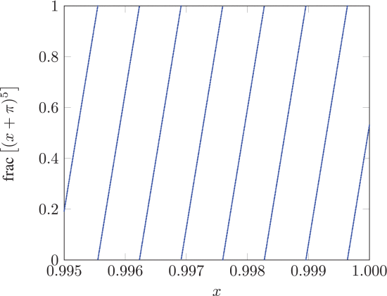
Figures 2, 3 and 4 show the zoom-in versions of the output of the original PRNG in (2). The geometrical visualization of application of the frac() part to Figure 1 consists of cutting the plot into pieces of height 1 and translating them down to the range [0,1).
It is possible to approximate a piece-wise continuous function with a DNN [8], [9].
A simplified version of this PRNG is helpful for the experimentation process:
![]() \begin{equation*}x_{n+1}=
\mathrm{f}\mathrm{r}\mathrm{a}\mathrm{c}
\left[\left(x_{n}+\frac{\pi}{3}\right)^{5}\right] \tag{3}\end{equation*}
\begin{equation*}x_{n+1}=
\mathrm{f}\mathrm{r}\mathrm{a}\mathrm{c}
\left[\left(x_{n}+\frac{\pi}{3}\right)^{5}\right] \tag{3}\end{equation*}
The experimentation with this simplified version of the PRNG provided some intermediate results and it also served as a starting point to solve the original version of the PRNG.
The PRNG in (2) is referred to as the original PRNG and the one in (3) the simplified PRNG.
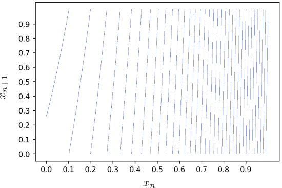
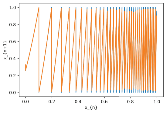
The simplified PRNG reduces the number of continuous segments of the output over the range [0,1) from 913 to 35. Its shape is shown in Figure 5 over the entire range of [0,1).
Experiments
The numbers of continuous segments of the original PRNG and the simplified PRNG differ by over an order of magnitude (from 913 to 35). Consequently the experiments for each of them use different DNN architectures and the preprocessing of the input also varies.
A. Simplified PRNG
The
complexity of the simplified PRNG already requires a DNN with many
nodes and layers to learn the model. But the PRNG has only one input, xn,
that proved insufficient to train the DNN. To solve this problem, a
preprocessing step was added to the system consisting of a
transformation from the one dimensional input to an 100-element vector:
![]() \begin{equation*}[x_{n},2x_{n},\ldots,34x_{n},x_{n}^{2},\ldots,x_{n}^{34},x_{n}^{-34},\ldots,x_{n}^{-2}] \tag{4}\end{equation*}
\begin{equation*}[x_{n},2x_{n},\ldots,34x_{n},x_{n}^{2},\ldots,x_{n}^{34},x_{n}^{-34},\ldots,x_{n}^{-2}] \tag{4}\end{equation*}
This strategy with increased dimension of input does not suffer from the curse of dimensionality [17], because all the input features in (4) lie on a twisted one-dimensional line in a one-hundred-dimensional space.
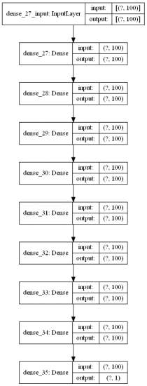
Figure 6 shows the architecture of the DNN consisting of 10 layers with 100 nodes each except for the output layer that has 1 node. These are dense layers, the weight initialization is orthogonal [18] and the bias initialization is 0.1. The activation function for all the layers uses a sigmoid, optimizer ADAM, and the loss function is the mean squared error. The DNN is trained with 3 million pseudo random numbers using a batch size of 35,000 during 38 hours on a NVIDIA GPU model GTX 2080 Ti.
B. Original PRNG
For the original PRNG, the one-dimensional input, xn, of the PRNG was preprocessed into a 512-element vector:
![]() \begin{equation*}\left[x_{n},
\text { frac }\left(x_{n}+\frac{1}{512}\right), \ldots, \text { frac
}\left(x_{n}+\frac{511}{512}\right)\right] \tag{5}\end{equation*}
\begin{equation*}\left[x_{n},
\text { frac }\left(x_{n}+\frac{1}{512}\right), \ldots, \text { frac
}\left(x_{n}+\frac{511}{512}\right)\right] \tag{5}\end{equation*}
The numbers of the vector in (4) sweep over a wide range. The vector in (5) restricts the range of the input on the unit interval while keeping the dimension of the input at 512. Note there is no raising the terms in (5) to the 5th power so no parametric hint is given to the DNN on the locations of the discontinuities in the PRNG. This choice of input worked well.
In the previous experiment, using the preprocessing of (4), it is observed that the training process starts by approximating all the predictions with a value around 0.5 and then slowly learns one segment piece at a time from left to right with high accuracy. The learning keeps going from left to right. The training process also presents diminishing returns. With the preprocessing of (5) the training is faster. Instead of learning slowly from left to right with diminishing returns, this preprocessing produces a faster learning pattern where all the pieces are learned simultaneously. The downside of the approach is a loss of accuracy.
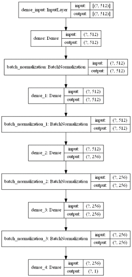
Figure 7 shows the architecture of the DNN consisting of 3 layers of 512 nodes, 2 layers of 256 nodes and the output layer of 1 node. All the layers, except for the input layer, are interspersed with batch normalization. They are dense layers, he weight initialization is orthogonal and the bias initialization is 0.01. The activation function for all the layers is sigmoid, optimizer ADAM and the loss function is the mean squared error. It is trained with 1 million sequential pseudo random numbers using a batch size of 35,000 during 3 weeks on a NVIDIA GPU model Tesla V100.
Analysis
Following the previous section, the results of the simplified PRNG and the original PRNG are analyzed here.
A. Simplified PRNG
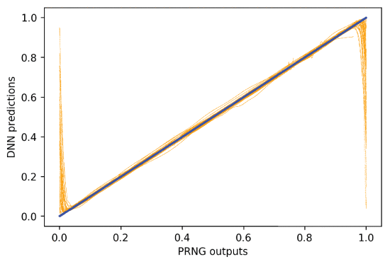
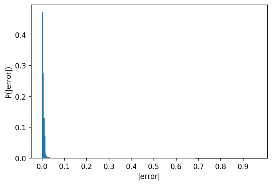
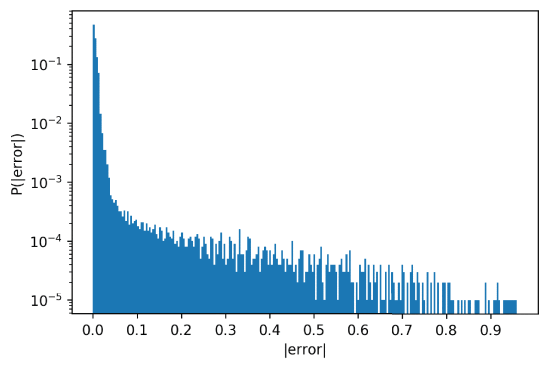
The mean square error (average of the squared errors) value on the trained DNN versus target value is about 0.00236. The results are shown in Figures 8, 9, 10 and 11. Figure 8 shows the DNN approximations in orange superimposed over the true pseudo random numbers in blue. The accuracy is such that the blue color is only visible close to the discontinuities. Figure 9 illustrates the displacement between the DNN predictions and the pseudo random numbers. Again, the approximations are clear except for the points closer to the discontinuities of the PRNG function. Figures 10 and 11 show the same histogram with 250 bins from 100,000 samples, on different scales, illustrating the distribution of the error of the approximations of the DNN. For almost half of the cases the error (magnitude) is less than 0.004, and about 90% of the numbers are approximated with an error less than 0.02. The error histogram in Figure 10 is shown on a more informative log scale in Figure 11.
B. Original PRNG
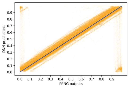
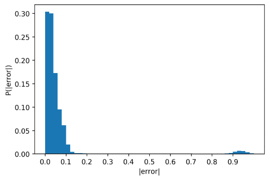
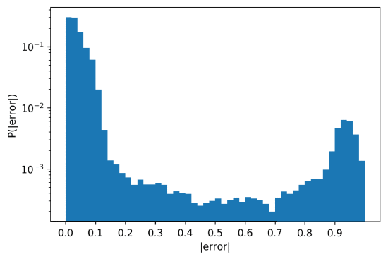
The mean square error of the trained DNN is 0.00261. The results are presented in Figures 12, 13 and 14. Figure 12 illustrates the displacement between the DNN predictions and the true pseudo random numbers. Figures 13 and 14 are the same histogram on different scales. They have 50 bins and were generated using 1,000,000 samples to illustrate the distribution of the error of the approximations of the DNN. For 60% of the cases the error is less than 0.04, and about 90% of the numbers are approximated with an error less than 0.1. The error histogram in Figure 13 is shown on log scale in Figure 14.
The primary sources of DNN error are seen graphically in Figure 9 where there are large variant spikes near 0 and 1. The same error is seen in Figure 12 where there are clouds shown in the upper left and lower right of the plot. Errors primarily arise from the sharp discontinuities in the PRNG. The discontinuities in (2) are evident in Figures 2 through 4. The training error for the simplified PRNG at the discontinuities is visible in Figure 8.
DNN predictions by PRNG outputs from 1,000,000 equidistributed numbers (simplified PRNG). The blue diagonal corresponds to zero error.
Here is an illustration of the source of these errors. A value of
DNN predictions by PRNG outputs from 1,000,000 equidistributed numbers (original PRNG). The blue diagonal corresponds to 0 error.
Conclusion
The modified linear congruential generator (LCG) can be mimicked by training a DNN. LCG’s are characterized by a piece-wise continuous function that can be learned by a DNN. Conventional DNN’s assume underlying continuity. The modified LCG in (2) consist of a non-linear piece-wise continuous function with many segments. We use DNN’s to approximate PRNG’s with tens and many hundreds of segments. It is a difficult task for DNN’s to learn functions with large amounts of jump discontinuities. Both theoretical and experimental work approximating non-linear functions with DNN’s is already available in the literature, as well as theoretical analysis on how DNN’s can approximate piecewise continuous functions. To our knowledge, this is the first article showing how a non-linear piece-wise continuous function with a multitude (913) of jump discontinuities can be approximated experimentally.
The ability of DNN’s to nonparametrically crack LCG’s and parametrically invert the more sophisticated Mersenne Twister makes one worry about the use of PRNG’s in the fields of cryptography and gaming. Better quantum random number generators that cannot be inverted should be used. 4


![Fig. 1. - A plot of $(x_{n}+\pi)^{5}$ over the interval [0, 1].](2021-Pseudo_files/amigo1-pa3-1570742721-small.gif)
![Fig. 2. - Original PRNG in (2) over the interval [0, 0.005].](2021-Pseudo_files/amigo2-pa3-1570742721-small.gif)
![Fig. 3. - Original PRNG in (2) over the interval [0.5, 0.505].](2021-Pseudo_files/amigo3-pa3-1570742721-small.gif)
