| |||||
| | |||||
The methods described so far attempt to identify nonessential elements by calculating the sensitivity of the error to their removal. The methods described next modify the error function so that error minimization effectively prunes the network by driving weights to zero during training. The weights may be removed when they decrease below a certain threshold; even if they are not actually removed, the network still acts somewhat like a smaller system.
As an aside, it should be noted that the simple heuristic of deleting small weights is just a heuristic. Obviously, if a weight is exactly zero, it can be deleted without affecting the response. In many cases, it may also be safe to delete small weights because they are unlikely to have a large effect on the output. This is not guaranteed, so some sort of check should be done before actually removing the weight. Input weights may be small because they're connected to an input with a large range; weights to output nodes may be small because the targets have a small range. These objections are less important when inputs and outputs are normalized to unit ranges, but there are cases where small weights may be necessary; a small nonzero bias weight may be useful, for example, to put a boundary near but not exactly at the origin. A more cautious heuristic would be to use the weight magnitude to choose the order in which to evaluate weights for deletion.
Figure 13.3 shows the change in error due to deletion of a weight versus the weight magnitude for a 10/3/10 network trained on the simple autoencoder problem (10 patterns where 1 of 10 bits is set). The graph gives some support to the heuristic because the smaller weights tend to give smaller changes in the error when the weight is deleted, but it also shows cases where smaller weights have more effect on the error than larger weights. THe graph shows two separate approximately linear trends. The upper-left group contains mostly hidden-to-output weights. In many networks, weights close to the output may be larger than weights close to the input because the delta-attenuation effect of back-propagating through intermediate node nonlinearilties causes input weights to grow slower.
Figure 13.3: Pruning error versus weight magnitude. One of the simplest pruning heuristics is that small weights can be deleted since they are likely to have the least effect on the output. Shown are the errors due to deletion of a weight versus weight magnitude for a 10/3/10 network trained on the simple autoencoder problem. There are two separate, approximately linear trends. The upper group contains input-to-hidden weights while the lower group contains hidden-to-output weights.
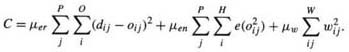
Chauvin [70], uses the cost function
where e is a positive monotonic function. The sums are over the set of output units, O, the set of hidden units H, and the set of patterns P. The first term is the normal sum of squared errors, the second term measures the average "energy" expended by the hidden units. The parameters uer and uen balance the two terms. The energy expended by a unit - how much its activity varies over the training patterns - is taken as an indication of its importance. If the unit activity has a wide range of variations, the unit probability encodes significant information: if the activity does not change much, the unit probability does not carry much information.Qualitatively different behaviors are seen depending on the form of e. Various functions are examined that have the derivative
where n is an integer. For n = 0, e is linear so high and low energy units receive equal differential penalties. For n = 1, e is logarithmic so low energy units are penalized more than high energy units. For n = 2, the penalty approaches an asymptote as the energy increases so high energy units are not penalized much more than medium energy units. Other effects of the form of the function are discussed by Hanson and Pratt [154].
A magnitude-of-weights term may also be added to the cost function, giving
Since the derivative of the third term with respect to wij is 2μwwij, this effectively introduces a weight decay term into the back-propagation equations. Weights that are not essential to the solution decay to zero and can be removed.
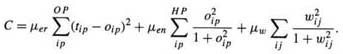
Solutions described in [72,73] use the cost function
No overtraining effect was observed despite long training times (with μer = .1, μen = .1, μw = .001). Analysis showed that the network was reduced to an optimal number of hidden units independent of the starting size.
Weigend, Rumelhart and Huberman [386,387,388] minimize the following cost function
where T is the set of training patterns and C is the set of connection indices. The second term (plotted in figure 13.4) represents the complexity of the network as a function of the weight magnitudes relative to the constant wo. At | wi| << wo, the term behaves like the normal weight decay term and weights are penalized in proportion to their squared magnitude. At | wi| >> wo, however, the cost saturates so large weights do not incur extra penalties once they grow past a certain value. This allows large weights which have shown their value to survive while still encouraging the decay of small weights.
The value of lambda requires some tuning and depends on the problem. If it is too small, it will not have any significant effect; if it too large, all of the weights will be driven to zero. Heuristics for modifying lambda dynamically are described.
Ji, Snapp, and Psaltis [195] modify the error function to minimize the number of hidden nodes and the magnitudes of the weights. They consider a single-hidden-layer network with one input and one linear output node. Beginning with a network having more hidden units than necessary, the output is
where ui and vi are, respectively, the input and output weights of hidden units i, theta_i is the threshold, and f is the sigmoid function.The significance of a hidden unit is computed by a function of its input and output weights
where sigma(w) = w^2 (1+w^2). This is similar to terms in the methods previously described.
The error is defined as the sum of Eo, the normal sum of squared errors, and E1, a term measuring node significances.
| (13.23) | 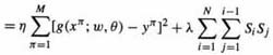 |
Conflict between the two error terms may cause local minima, so it is suggested the second term be added only after the network has learned the training set sufficiently well. Alternatively, lambda can be made a function of E0 such that
When E0 is large, lambdaλ will be small and vice versa.
A second modification to the weight update rule explicitly favors small weights
The new tanh(.) term is modulated by μ:
This reduces u gradually and makes it go to zero when the target-value vomponent E0 of the error function ceases to change,Once an acceptable level of performance is achieved, small magnitude weights can be removed and training resumed. It was noted that the modified error functions increase the training time.
Many of the penalty term methods include terms that effectively introduce weight decay into the learning process, although the weights don't always decay at a constant rate. The third term in equation 13.17, for example, adds a -2μwwij term to the update rule for Wij. This is a simple way to obtain some of the benefits of pruning without complicating the learning algorithm much. A weight decay rule of this form was proposed by Plaut, Nowlan, and Hinton [299].
Ishikawa[187] proposed another simple cost function
The second term adds -λ sgn(Wij) to the weight update rule. Positive weights are decremented by λ and negative weights are incremented by λ.
A drawback of x xxxxxxxx xx xxx xxxxxxx xxx xxxxxxx xxxx xx xxxx xx xxxxx xx xxxxx xxxxxx xxxxxxx xxxx xxxx xxxxx xxxxxxxxxx xxxx xxxxxxx xxxx x xxxxxx xxxxx xxxxxxxxxx xxxx xxxx xxxx xx xx xxxxxxxxx xxxxxxx xxx xxxxxx xxxxxxxxxxx xxxx xx xxxxxxxx xxxxx xxxxxxxxx xxxx xx xxxxxx xxx xxxxxxx xxxxxxxx xxxx x xxxxxxx xxxxxx xxxxxx xxx xxxxxx xxxxx xxxxxxxx xxxx xxxxxx xxxxxxxx xxxxx xxxx x xxxx xxxxxxx xxxxxxx xxxx xxxxxxxx xxx xxxxx xxxxxxxxxxx xxxxxxxxxxxx xx xxx xxxxxxx xx x xxxxxxx xx xxxxxxxxxx xxxxxxxx xxxx xx xxxxxxx xxxxx xxxx xxxxxxxxxxxx xxxx x xxxxxx xxxxx xx xxx xxxxxxx xxxx xx xxxxxxx xx xxx xxxxxxxxxxxx xxxxxx xxxxxxxxx xx xxx xxxxxxxxxxxx xxxxxxxx xx xxx xxxxxxxxxx xxx xxxxxxxx xxx xxxxxx xxx xxx xxxxxx xxxx xxxxxxxx xx xxxx xxxx xxxxxxxxxxxxx xxxxx xxxxxx xxxxxxxxxxxx xxxx xxx xxxxxx xxxxxxxx xxxxxx x xxxxxx xxxxx xxxxxxxxxx xxx xxxxx xxxxxxx xx xxxxx xxxxxx xxxxxxxx xxxxxxxx xxx xxxx xxxxxxxxxx xx xxx xxxxxx xxxxxxxx xxx xx xxxx xxxx xxx xxxxxx xxxxx xx xxx xxxxx xxxxxxxxx xx xxxxxxxxx xxxx xxxx xxx xxxxxxxxx xxx xxxx xxx xxxxx xxxxxxx xxx xxxxxxx xxx xxxx xxxxxxx xx xxxxxxxx xxx xxxx xxxxxxxx xxxxxx
Bias Weights Some authors suggest that bias weights should not be subject to weight decay. In a linear regression y = wTx + θ, for example, the bias weight θ compensates for the difference between the mean value of the output target and the average weighted input. There is no reason to prefer small offsets, so θ should have exactly the value needed to remove the mean error.
xx x xxxxxxxxx xxxx xxxxxxxx x x xxxxx x xxxxxxxx xxx xxxx xxxxxx xxx xxx xxxxxx xx xxxxxxxx xxx xxxxxxxx xxxxxxxx xx xxx xxxxx xxxxxx xx xxxx xxx xxxxxx xxxxxxx xxx xxx xxxx xxx xxxxxx xx xxx xxxx xxxxxx xxxxxxx xxxx xxx xxxxxxxx xx xxx xxxxxxxx xxxxxxx xxxxx xxxxx xxxxx xx xxx xxxxxxx xxxxxxxxxx xxxxxxx xx xxx xxxx xxxxxx xx xxx xxxxxxx xx xxxxx xxxxxx xxx xxxxxxxx xxxxxx xx xxx xxxxxxx xxxxxxx xxx xxxxxxxx xx xxx xxxxxxxx xxxx xxx xxxxxx xx xxxxxxxxx x xxx xxxxx x xxxxxxxx xxx xxxx xxxxxxx xxxxxxxxx xx xx x xx xx xxxxxx xxxxx xxxxx xxxxx xxx xxxxxxxx xxxx xxxx xxx xxxxxx xx xxx xxxx xxxx xx xxxxxxx xxx xxxxxx xxxx xxxxxxxx xxxx xxxx xxxxxxx xxxxxx xx xxxxxxx xx xxxxxx xx xxxxx xxx xxxxxxxxx xxxxxx xxxxxx